Ordinary differential equations (ODE)
Example 1: Solving scalar equations
In this example, we will find the function u(t) which satisfies
\[\frac{du}{dt} = \alpha \cdot u\left( t \right) = 1.01 \mathrm{ \textcolor{#15a}{s{^-}{^1}}} \cdot u\left( t \right)\]\(\left( 0 \mathrm{ \textcolor{#15a}{s}} \leq t \leq 2 \mathrm{ \textcolor{#15a}{s}} \right)\)
This 'hello world' of ODEs is solved analytically by brilliantly pulling from calculus that if \(u\left( t \right) = c{_1} \cdot e^{\alpha \cdot t}\), then \(\frac{du}{dt} = c{_1} \cdot \alpha \cdot e^{\alpha \cdot t}\). We plug in our initial condition:
\[u\left( 0 \mathrm{ \textcolor{#15a}{s}} \right) = c{_1} \cdot \alpha \cdot e^{\alpha \cdot 0 \mathrm{ \textcolor{#15a}{s}}} = c{_2} = 0.5 \mathrm{ \textcolor{#15a}{m}}\] ...and the solution is \[u\left( t \right) = 0.5 \mathrm{ \textcolor{#15a}{m}} \cdot e^{\alpha \cdot t} = e^{1.01 \mathrm{ \textcolor{#15a}{s{^-}{^1}}} \cdot t}\]
Or, we can ask the computer in computer language. Leibniz notation can't be used as a variable name for the derivative, so we switch to Lagrange notation, u´:
import MechanicalUnits: @import_expand, dimension
@import_expand(mm, cm, m, km, ft, inch, s, °, kg)
using MechGluecode
using DifferentialEquations, Plots, ArrayTools
plotly()
Plots.PlotlyBackend()
u´(u,p,t) = 1.01s⁻¹ * u
const uᵢ = 0.5m
prob = ODEProblem(u´, uᵢ, (0.0, 2)s)
sol = solve(prob)
default(width = 5, framestyle = :zerolines, legend=(0.15, 0.9),
    foreground_color_legend = nothing, background_color_legend = nothing)
plot(sol, label = "Interpolation curve")
scatter!(sol.t, sol.u, marker=true, linewidth=0, label="Exact points")
last_plot_with_data_to_html("output/script02.html")And the default solution plots like:
A few remarks:
The plot will be more informative if we label the vertical axis 'Distance u(t) [m]' and the horizontal axis 'Time t [s]'. But we get the unit labels for free since they are contained in the solution. They often provide enough information for interpreting what the curves represent.
The numerical solver uses only four numerical steps here. It is able to pick interpolation functions which match perfectly.
We do not need to specify the solution algorithm, although that is recommended. Inspect
solto find which algorithm was found to be the best here.The first parameter in u´(u, p, t), is the function u(t), the one we want to find.
We do not use the second parameter, p here.
Differentialequations.jlwill treat any three-parameter function in the same way: The second parameter will be used for parameters that do not vary with the integration variable. In our case, we're just interested in one constant value, α = 1.01 /s , but we could have passed α as argument p for more flexibility.The third parameter, t, is used in non-homogenous problems but we don't use it here. It is the argument to u, but for homogenous problems, the relationship between u(t) and u´(t) is the same, regardless of t.
Example 2: Termination criterion
Above, we decided in advance where on the t axis we would stop the numerical integration. We will now stop when u reaches targval = 1.0
m
. DifferentialEquations.jl will look for a function which returns unitless zero.
const targval = 1.0m
condition(u,t,integrator) = (u - targval) / m
affect!(integrator) = terminate!(integrator)
cb = ContinuousCallback(condition, affect!)
solstop = solve(prob,Tsit5(), callback=cb)
plot!(solstop, xlims = (0,2)s,
    label = "Solve process stopped at $targval",
    linewidth = 8, color=:black)
scatter!(solstop.t, solstop.u, marker=true, linewidth=0,
    label="Exact points, stopped at $targval")
last_plot_with_data_to_html("output/script03.html")Callback functions like this can be used for progress meters, making balls bounce, or sliding support conditions on a non-linear beam. See Event handling and callback functions.
We normally tell solve which solution algorithm to use, in this case Tsit5() (Tsitouras, Ch). For small problems, most of the 'solve' time may easily be spent picking the best algorithm. When defining specific algorithms, you could do with loading fewer dependencies. Using binary dependencies can be a pain due to the security policies many institutions apply, and they increase load times.
Example 3: Simple variation of parameters
In examples 1-3, we used a hard-coded α = 1.01 s⁻¹ . We can pass the value as function parameter α instead. The interface does not care if the parameter is called p or α as long as it's in the correct position.
u´(u,α,t) = α * u
function time_to_targval(p)
    sol = solve(prob, Tsit5(); callback=cb, p = p)
    sol.t[end]
end
@time plot(time_to_targval, xlims = (1.00000/s, 1.5/s), xguide ="Parameter α",
    label = "Time to reach $targval")
last_plot_with_data_to_html("output/script04.html") 1.227606 seconds (1.80 M allocations: 104.176 MiB, 2.05% gc time, 99.82% compilation time)
To make this plot, the differential equation solver runs hundreds of times. We do not specify how many, just naively pass the function to the plotting engine. We are patient.
Example 4: Big gun - system of differential equations
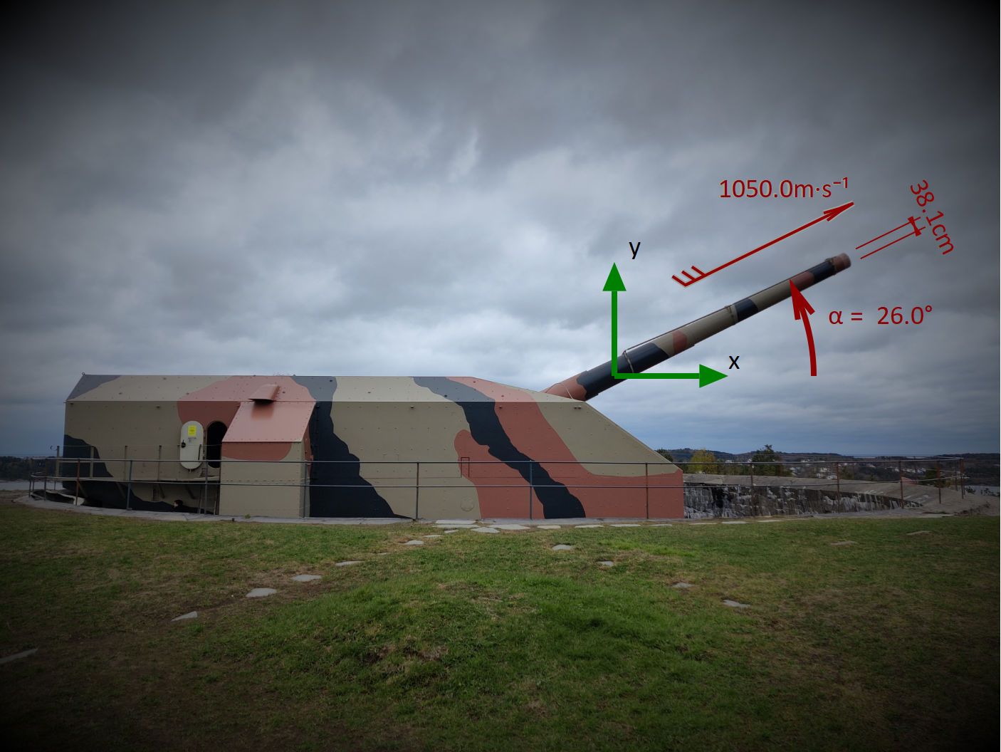
In two minutes, this gun could shoot five cannonballs the weight of my first car. The long-distance balls are just 495 kg - could they shoot across the Skagerrak?
No air resistance
import MechanicalUnits: g, ∙
"Barrel elevation"
α₀()  = 26°
"Muzzle velocity"
v₀()  = 1050m/s
let
    Δt = 2 * v₀() * sin(α₀()) / g
    Δx =  v₀() * cos(α₀()) * Δt
    println("Time until impact, Δt   = ", round(s, Δt))
    println("Horizontal distance, Δx = ", round(km, Δx))
end
Time until impact, Δt = 94.0s
Horizontal distance, Δx = 89.0km
Without air resistance, the gun would shoot from Møvig to Denmark at this angle. We skipped straight to the known answer here, but as a reminder:
\[y'' = v' = a = - g\]That's a second order differential equation, and we could have used separation of variables to create a system of first order ODEs. Just not a very interesting one, because we will not get a good estimation without also considering air resistance along both x and y axes.
Why the parantheses? Why write α₀() when
const α₀would work? It's a working habit. We can easily revise functions when we are detailing the model more and more.
Air resistance and sound barrier effects
In the bunkers below, there is still an analogue computer with magic-level mechanics. It is able to target ships at roughly 50 km, or about three times the distance you would be able to see a large ship over the horizon. Let us go a step further towards that magic and introduce the magnitude of air resistance R.
\[R = 0.5 \cdot \rho{_0} \cdot C_{s} \cdot A_{pr} \cdot v^{2}\]Cₛ is aerodynamic shape coefficient as a function of Mach number
Aₚᵣ is projected frontal area, projectile
v is velocity
The Mach number, M is the ratio of velocity v to local speed of sound c. The sound barrier heavily influences the flow. We are interpolating data from figure 3 in (Lipanov, Korolev, Rusyak (2017)), where an advanced model is discussed. The shape coefficient Cₛ function is
\[\mathrm{C_{s}}\left( v, c \right) = \mathrm{C_{s}}\left( \frac{v}{c} \right) = \mathrm{C_{s}}\left( v_{ma} \right)\]\(c = 323\) m/s is the speed of sound at ground level
The velocity and resistance are 2d vectors in our problem of course. We define the functions in detail like this:
using Interpolations
using MechanicalUnits: Velocity, Density
# Constants we don't think we'll change
const x₀ = 0.0km
const y₀ = 0.0km
const ø = (1900//127)inch

# Calculated constants
const Aₚᵣ = π/4 * ø^2

# 'Constants' that we might want to modify later
mₚ()   = 495kg
x´₀() = v₀() * cos(α₀())
y´₀() = v₀() * sin(α₀())
c() = 323.0m/s
ρ() = 1.225kg/m³

# Functions of current velocities
const ptsM = [0, 0.5, 0.75, 0.875, 1, 1.125, 1.25, 1.5, 2, 2.5, 3.0]
const ptsCd = [0.155, 0.16, 0.165, 0.17, 0.2575, 0.3875, 0.3775,
                0.3425, 0.2875, 0.245, 0.215]
Cₛ(vₘₐ::Real) = LinearInterpolation(ptsM, ptsCd, extrapolation_bc=Flat() )(vₘₐ)
Cₛ(v::T, c::T) where T<:Velocity =  Cₛ(v / c)
v(vx, vy) = √(vx^2 + vy^2)
R(v::T, c::T, ρ::Density) where T<:Velocity = 0.5∙ρ∙Cₛ(v, c)∙Aₚᵣ∙v^2
α(vx, vy) = atan(vy, vx)
Rx(vx, vy, c, ρ) = R(v(vx, vy), c, ρ) * cos(α(vx, vy))
Ry(vx, vy, c, ρ) = R(v(vx, vy), c, ρ) * sin(α(vx, vy))
plot(Cₛ, xlims = (0,3), label = :none,
    yguide = "Shape coefficient, Cₛ []", xguide = "Mach number, vₘₐ []",
    title = "Interpolation curve,  Cₛ(vₘₐ)" )
last_plot_with_data_to_html("output/script06.html")In earlier examples, we are solving for a scalar valued function u:R ↣ R with scalar domain, time. Our new function Γ:R ↣ R⁴ still has single input, a real quantity with dimension time. The function values represent two position coordinates (x, y) and two corresponding velocities (x´, y´) . Engineers might call this sort of structure a local tuple, Γ (Gerald Jay Sussman and Jack Wisdow (2015)), and would say we have two degrees of freedom. Matematicians would perhaps say we have four degrees of freedom. What would you say? Leave a a comment below, but you can't.
Instead of defining u'(t) which returns the current derivative of u, the derivatives are now output as an updated first argument. This is faster because we avoid heap memory allocation for every iteration. Differentialequations.jl understands our intention from the number of function parameters. So with four arguments, the first argument is actually our output. In Julia, the custom is also to add an '!' to the name of in-place functions. DifferentialEquations.jl simply counts the number of non-keyword arguments and treats the function as in-place ('!') or, ehem, out-of-place accordingly.
"""
    Γ₁!(Γ´, Γ´, p, t)
Local tuple with derivatives. p and t are not used.
"""
function  Γ₁´!(Γ´, Γ, p, t)
    (x, y), (x´, y´) = packout(Γ)
    @debug "Γ"    x    y    x´   y´   maxlog = 2
    x´´ =     -Rx(x´, y´, c(), ρ()) / mₚ()
    y´´ = -1g -Ry(x´, y´, c(), ρ()) / mₚ()
    @debug "Γ Acceleration"    x´´|> g    y´´|>g    maxlog = 2
    packin!(Γ´, x´, y´, x´´, y´´)
end
Feel free to skip the @debug lines. The cost, in addition to some ugliness, is 20 ns of execution time.
Why do we use the pakin and packout functions (defined below), when Parameterized functions has really nice ways of doing this without the clutter? Well, there are
Three Steps to Computational Bliss:
Correct syntax
Type stable functions
Inferrable type functions
Arguments u and u´ are now going to hold quantities with different dimensions, meaning they can't be represented with the exact same type. We might, inadvisably, pack the elements in Vector types.
However, when we cram elements with different types into a normally type-uniform Vector, the compiler may have a hard time figuring out the exact types of those elements. The internal type description of an easy-to-type function might be Vector{Quantity{Float64, D, U} where {D, U}}. Here, the Dimension and Unit is undetermined. We saved on thinking and typing, but the compiler might spend minutes inferring the exact machine code before running.
Instead, we'll organize by unit type with ArrayPartition, imported from RecursiveArrayTools:
"Local tuple initial condition"
Γ₀() = ArrayPartition([x₀, y₀], [x´₀(), y´₀()])

packout(Γ) = Γ.x[1], Γ.x[2]
function packin!(Γ´, x´, y´, x´´, y´´)
    Γ´.x[1][1] = x´;  Γ´.x[1][2] = y´
    Γ´.x[2][1] = x´´; Γ´.x[2][2] = y´´
    return Γ´
end
We prefer a fixable error to a slow run, so we define the function solve_guarded before trying this out. It will check that our model is actually inferrable (i.e. 'hundreds of times faster', at least in some cases).
using Logging: disable_logging, LogLevel, Debug, with_logger
import Logging
using Test: @inferred
# Exit criterion - hit sea level
function terminate_condition(Γ, t, integrator)
    (_, y), (_, _) = packout(Γ)
    y / m
end

cb1 = ContinuousCallback(terminate_condition, affect!)

function solve_guarded(Γ´!;  Γᵢₙ = Γ₀(), alg = Tsit5(), debug=false)
    # Test the functions
    @inferred packout(Γᵢₙ)
    @inferred packout(0.01Γᵢₙ/s)
    @inferred Γ´!(Γᵢₙ/s, Γᵢₙ, nothing, nothing)
    # Define and solve
    prob = ODEProblem(Γ´!, Γᵢₙ, (0.0s, 200s))
    sol = if debug
        with_logger(Logging.ConsoleLogger(stderr, Logging.Debug)) do
            solve(prob, Tsit5(), callback = cb1)
        end
    else
        solve(prob, Tsit5(), callback = cb1)
    end
    sol
end

sol₁ = @time solve_guarded(Γ₁´!, debug=true);
┌ Debug: Γ
│ x = 0.0km
│ y = 0.0km
│ x´ = 943.7337486141254m∙s⁻¹
│ y´ = 460.2897041285313m∙s⁻¹
└ @ Main C:\Users\f\.julia\environments\sandbox3\script07.jl:7
┌ Debug: Γ Acceleration
│ x´´ |> g = -3.064765825228892g
│ y´´ |> g = -2.494786169287076g
└ @ Main C:\Users\f\.julia\environments\sandbox3\script07.jl:10
The plots above show parameters that are not directly part of the solution. They are just necessary for reasonability checking. Extracting indirect parameters is more tedious, as can be seen below. A better approach might be to include speed and air resistance as directly coupled DOFs. If we did, they could be interpolated directly from the solution object without all of this code:
function time_distributed_motion_vals(;sol = sol₁, Γ´! = Γ₁´!)
    ts = range(sol.t[1], sol.t[end], length = 300)
    xs = map(t->sol(t).x[1][1], ts)
    ys = map(t->sol(t).x[1][2], ts)
    x´s = map(t->sol(t).x[2][1], ts)
    y´s = map(t->sol(t).x[2][2], ts)
    vs = map(hypot, x´s, y´s)
    Γs = map(sol, ts)
    dummyΓ´ = Γs[1] / (ts[2]- ts[1])
    x´´s = [Γ´!(dummyΓ´, Γ, nothing, nothing).x[2][1] |> g for  Γ in Γs]
    y´´s = [Γ´!(dummyΓ´, Γ, nothing, nothing).x[2][2] |> g for  Γ in Γs]
    as = map(hypot, x´´s, y´´s)
    ts, xs, ys, vs, as
end
function plotvals₁()
    ts, xs, ys, vs, as = time_distributed_motion_vals()
    Cₛs = map(v->Cₛ(v, c()), vs)
    ρs = repeat([ρ()], length(Cₛs))
    xlims = (0.0km, maximum(xs))
    ts, xs, ys, vs, as, Cₛs, ρs, xlims
end
function bulletplots(f;  trajectory_label = "Constant atmosphere α₀ = $(round(°, α₀()))",
        p_y_x = plot(), p_v_x = plot(), p_v = plot(), p_Cρs= plot(), p_a= plot(),
        kw...)
    ts, xs, ys, vs, as, Cₛs, ρs, xlims = f()
    plot!(p_y_x, xs, ys, xguide="x",
        yguide ="y", label = trajectory_label; xlims, kw...)
    plot!(p_v_x, xs, vs, xguide ="x",
        yguide ="v"; xlims, label = trajectory_label, kw...)
    plot!(p_v, ts, vs, yguide = "v"; label = trajectory_label, kw...)
    plot!(p_Cρs, [ts ts], [Cₛs ρs], yguide = "Cₛ, ρ", color = ["Red" "Black"] ;
        label = trajectory_label,  kw...)
    plot!(p_a, ts, as, yguide = "a", color = "Green", xguide = "Time",
        label = trajectory_label; kw...)
    return p_y_x, p_v_x, p_v, p_Cρs, p_a
end

# Subplots
p_y_x, p_v_x, p_v, p_Cρs, p_a = bulletplots(plotvals₁; linestyle=:dot)

# Assemble subplots
p_v_Cs_a = plot(layout = (3, 1), p_v, p_Cρs, p_a, legend=false)
p_y_x_v = plot(layout = (2, 1), p_y_x, p_v_x, legend=false)
last_plot_with_data_to_html("output/script10a.html")
last_plot_with_data_to_html("output/script10b.html")
Modifying the shot model - atmospheric properties ODE
We have a simple model that we can thrust, but check. Much of the model can be reused while we also add a bit more realism.
Most importantly on this scale, air density depends on altitude, but also on humidity and temperature. We can reduce that to just elevation by using the international standard atmosphere. And who could have known, the standard is also formulated as an ODE!
\[\frac{dp}{dy} = - {\rho}g\]The local speed of sound, c, also varies linearly in the troposphere and is based on the same constant quantities. The sound barrier heavily influences drag for this big bullet.
\[c = \sqrt{\gamma \cdot R_{s} \cdot T}\]The therodynamics details are collapsed below, constants are summarized in the table. The resulting functions will become part of the extended ODE.
The solution to (7) is
psol, which is a global variable here, although it can be called like a normal function:psol(y). To make this inferrable, we can put in a crash barrier, an exact type warranty to the compiler. Voilà,p(y)is inferrable. Which we want, that's the third step after all. Alternatively, we could defineconst psol = ...., which would lead to irritating redefinition warnings or errors.
# Celsius temperature is affine, special treatment
import MechanicalUnits: °C
@import_expand(K, J, kPa)
"Gas constant, dry air (other source)"
const Rₛ =  287J∙kg⁻¹∙K⁻¹
"Base geopotential altitude"
const yₐ₀ = -610m
"Top of troposphere, geopotential altitude"
const yₐ₁ = 11km
"Base temperature"
const T₀ = 19°C
"Top of troposphere, temperature"
const T₁ = -56.5°C
"Base pressure"     ps
const p₀ = 108.9kPa
"Adiabatic constant cp/cv, troposphere"
const γ = 1.26

"Temperature in troposphere and tropopause"
T(y) = y < yₐ₁ ? T₀ + (y-yₐ₀)∙(T₁-T₀) / (yₐ₁-yₐ₀) : K(T₁)

println(lpad("At sea level, standard temperature = ", 52),
    round(°C, T(0m)   , digits = 2))

"Density as a function of pressure and temperature"
ρ(p, T) = p / (Rₛ∙(T |> K)) |> kg/m³
println(lpad("Air density ρ(p = 101kPa, T = 15.0°C) = ", 52),
    round(kg/m³, ρ(101kPa, 15.0°C), digits =3))

"Pressure derivative with respect to geopotential altitude"
p´(p, notused, y) = -ρ(p, T(y))∙g |> kPa/km

println(lpad("Pressure derivative with respect to altitude, 0m) = ", 52),
    round(kPa/km, p´(101kPa, nothing, 0m), digits= 2))
"Pressure solution with respect to geopotential altitude"
psol = solve(ODEProblem(p´, p₀, (y₀, 25.0km)), Tsit5())
"Pressure as a function of altitude, with exact type warranty"
p(y) = kPa(psol(y))::typeof(1.0kPa)
println(lpad("Pressure derivative with respect to altitude, 0m) = ", 52),
    round(kPa/km, p´(101kPa, nothing, 0m), digits= 2))
"Pressure solution with respect to geopotential altitude"
psol = solve(ODEProblem(p´, p₀, (y₀, 25.0km)), Tsit5())
println(lpad("Pressure at top of troposphere is p(y = 11km) = ", 52),
    round(kPa, p(11.0km), digits = 2))
println(lpad("Pressure at bottom of stratosphere is p(y = 20km) = ", 52),
    round(kPa, p(20.0km), digits = 2))
"Density as a function of altitude"
ρ(y) = ρ(p(y), T(y))
println(lpad("Air density ρ(y = 11km) = ", 52),
    round(kg/m³, ρ(11km), digits = 4))
println(lpad("Air density ρ(y = 20km) = ", 52),
    round(kg/m³, ρ(20km), digits = 4))
"Speed of sound"
c(y) = sqrt(γ∙Rₛ∙T(y)) |> m/s
let # For plot
    ys = range(0, 25, length = 50)km
    ρs = map(ρ, ys)
    cs = map(c, ys)
    plot([ρs cs],  [ys ys], yguide = "Altitude, y [km]",
        layout = (1, 2), label = :none)
        # Recipe don't work well with subplots
    plot!(xguide = ["Density [kg/m³]" "Speed of sound [m/s]"])
end
last_plot_with_data_to_html("output/script11.html")
At sea level, standard temperature = 15.03°C
Air density ρ(p = 101kPa, T = 15.0°C) = 1.221kg∙m⁻³
Pressure derivative with respect to altitude, 0m) = -11.98kPa∙km⁻¹
Pressure at top of troposphere is p(y = 11km) = 24.32kPa
Pressure at bottom of stratosphere is p(y = 20km) = 5.88kPa
Air density ρ(y = 11km) = 0.3911kg∙m⁻³
Air density ρ(y = 20km) = 0.0946kg∙m⁻³
| Constant quantity | Name and value |
|---|---|
| Gas constant, dry air (other source) | Rₛ = 287J∙kg⁻¹∙K⁻¹ |
| Base geopotential altitude | yₐ₀ = -610m |
| Top of troposphere, geopotential altitude | yₐ₁ = 11km |
| Base temperature | T₀ = 19°C |
| Top of troposphere, temperature | T₁ = -56.5°C |
| Base pressure | p₀ = 108.9kPa |
| Adiabatic constant cp/cv, troposphere | γ = 1.26 |
Time to define, solve and plot version 2 - now with altitude sensitivity!
function  Γ₂´!(Γ´, Γ, p, t)
    (x, y), (x´, y´) = packout(Γ)
    @debug "Γ"    x    y    x´   y´   maxlog = 2
    x´´ =     -Rx(x´, y´, c(y), ρ(y)) / mₚ()
    y´´ = -1g -Ry(x´, y´, c(y), ρ(y)) / mₚ()
    @debug "Γ Acceleration"    x´´|> g    y´´|>g    maxlog = 2
    packin!(Γ´, x´, y´, x´´, y´´)
end

sol₂ = solve_guarded(Γ₂´!);

function plotvals₂(;sol = sol₂, Γ´! = Γ₂´!)
    ts, xs, ys, vs, as = time_distributed_motion_vals(;sol, Γ´!)
    Cₛs = map(zip(vs, ys)) do (v, y)
        Cₛ(v, c(y))
    end
    ρs = map(ρ, ys)
    xlims = (0.0km, maximum(xs))
    ts, xs, ys, vs, as, Cₛs, ρs, xlims
end

# # Subplots, solid lines, overlaid on the previous, dashed
bulletplots(plotvals₂;
    trajectory_label = "α₀ = $(round(°, α₀()))",
    p_y_x, p_v_x, p_v, p_Cρs, p_a)
# Assemble subplots
p_v_Cs_a₂ = plot(layout = (3, 1), p_v, p_Cρs, p_a, legend=false)
p_y_x_v₂ = plot(layout = (2, 1), p_y_x, p_v_x, legend=false)
last_plot_with_data_to_html("output/script12a.html")
last_plot_with_data_to_html("output/script12b.html")
The solid lines are from model 2. The thinner air higher up is important!
Varying initial conditions
Similar guns on Bismarck and Tirpitz, two war ships, were limited to an elevation of 30°. But as we have seen, there is less resistance in the upper skies, so these land-mounted guns can shoot up to 60°.
const αᵢₙ₃ = (26:60)°
const Γᵢₙ₃ = [ArrayPartition([x₀, y₀], [v₀() * cos(α), v₀() * sin(α)])
                for α in αᵢₙ₃]
const sols₃ = [solve_guarded(Γ₂´!;  Γᵢₙ) for Γᵢₙ in Γᵢₙ₃]
p_y_x, p_v_x, p_v, p_Cρs, p_a = plot(), plot(),plot(),plot(),plot()

for (α₀, sol) in zip(αᵢₙ₃, sols₃)
    foo = () -> plotvals₂(;sol)
    bulletplots(foo;
        trajectory_label = "α₀ = $(round(°, α₀))",
        p_y_x, p_v_x, p_v, p_Cρs, p_a, legend=true)
end
# Assemble subplots
p_v_Cs_a₂ = plot(layout = (3, 1), p_v, p_Cρs, p_a, legend=false, linewidth = 1)
p_y_x_v₂ = plot(layout = (2, 1), p_y_x, p_v_x, legend=false, linewidth = 1,
        xlims = (0,55))
last_plot_with_data_to_html("output/script13a.html")
last_plot_with_data_to_html("output/script13b.html")
It is fair to say that this gun reaches out of the atmosphere to shoot farther. The advertised range of 55 km seems reasonable (some sources state 49.0 km ). Albeit at an elevation angle of 54° and a flight time of 130 s , precision may be compromised. Aiming precision data could be collected from online sources or inspected in the museum.
The calculation time for that last group of shots is 1.5 s on a 2020 computer, with no parallelism in use.
References
** Tsitouras, Ch** Runge–Kutta pairs of order 5 (4) satisfying only the first column simplifying assumption., Computers \& Mathematics with Applications, Elsevier, 2011.
Sussman, Wisdom Structure and Interpretation of Classical Mechanics, 2nd ed., 2015.
Lipanov, Korolev, Rusyak AIP Conference Proceedings 1893, 030085 (2017); Optimization of aerodynamic form of projectile... https://doi.org/10.1063/1.5007543.